GMM Forward-Looking Analysis

Indicatori di Fiducia delle Imprese per Modelli GMM

Istat

Fiducia delle imprese

Econometria

Gli indicatori Istat di fiducia delle imprese preparati per modelli GMM forward-looking: dataset disponibili e prime analisi.

Autore/Autrice

Paolo Volterra

Data di Pubblicazione

5 febbraio 2026

Sommario

Questo notebook presenta il dataset consolidato per analisi GMM (Generalized Method of Moments) forward-looking utilizzando indicatori di fiducia delle imprese e consumatori. Fonte dati: Eurostat (DG ECFIN) + Istat (DCSC_IESI)

Parole chiave

GMM, econometria, modelli, Istat, Eurostat, fiducia, imprese, ESI, IESI, LookingForward, previsioni

Gli indicatori di fiducia sono leading indicators ideali per modelli forward-looking perché:

Catturano aspettative degli agenti economici
Anticipano variabili macroeconomiche reali (PIL, produzione, occupazione)
Disponibili mensilmente con bassa latenza
Forniscono strumenti validi per GMM

1 Dataset Disponibili

1.1 Files generati

File	Descrizione	Dimensioni
`data_panel_long.parquet`	Panel base formato long	49,757 obs × 10 var
`data_panel_wide.parquet`	Panel base formato wide	963 obs × 9 var
`data_panel_integrated.parquet`	Panel con dati Istat integrati	5,939 obs
`data_panel_gmm_ready.parquet`	Panel GMM-ready con tutte le trasformazioni	49,757 obs × 27 var

1.2 Copertura dati

Paesi: Italia, Germania, Francia, Spagna, Area Euro (EA20)
Periodo: 2010-01 → 2026-01 (16 anni, frequenza mensile)
Indicatori: 6 serie per paese
- Economic Sentiment Indicator (ESI) - composito
- Industry confidence
- Services confidence
- Construction confidence
- Retail trade confidence
- Consumer confidence

1.3 Trasformazioni GMM incluse

Il dataset data_panel_gmm_ready.parquet include:

Lag variabili (t-1, t-3, t-6, t-12)
Differenze (prima e seconda)
Tassi di variazione (mensili e annuali)
Medie mobili (3, 6, 12 mesi)
Gap vs benchmark (differenza da EA20)
Variabili strutturali (entity_id, time_id, year, month, quarter)

Codice

import pandas as pd
import numpy as np
import matplotlib.pyplot as plt
import seaborn as sns

# Carica panel GMM-ready
panel = pd.read_parquet('data_panel_gmm_ready.parquet')

print(f"📊 Panel GMM-Ready")
print(f"   Dimensioni: {panel.shape}")
print(f"   Paesi: {panel['country_code'].unique()}")
print(f"   Indicatori: {panel['indicator'].unique()}")
print(f"   Periodo: {panel['time'].min().date()} → {panel['time'].max().date()}")

panel.sample(5)

📊 Panel GMM-Ready
   Dimensioni: (49757, 27)
   Paesi: <ArrowStringArray>
['DE', 'EA20', 'ES', 'FR', 'IT']
Length: 5, dtype: str
   Indicatori: <ArrowStringArray>
['construction', 'consumer', 'industry', 'retail', 'sentiment', 'services']
Length: 6, dtype: str
   Periodo: 2010-01-05 → 2026-01-05

	time	country_code	country_name	value	indicator	dataset_code	indic_code	indicator_label	unit_code	unit_label	...	value_growth12	value_ma3	value_ma6	value_ma12	gap_value	entity_id	time_id	year	month	quarter
9733	2022-02-05	DE	Germany	15.3	services	ei_bsse_m_r2	BS-SARM	Evolution of demand over the past 3 months	BAL	Balance	...	17.692308	18.933333	15.700000	14.266667	4.333333	DE_services	147	2022	2	1
14045	2021-12-05	EA20	Euro area – 20 countries (2023-2025)	36.0	consumer	ei_bsco_m	BS-PT-NY	Price trends over the next 12 months	BAL	Balance	...	-11.330049	27.266667	7.183333	3.533333	NaN	EA20_consumer	145	2021	12	4
12139	2024-09-05	EA20	Euro area – 20 countries (2023-2025)	14.1	construction	ei_bsbu_m_r2	BS-FLBA3-PC	Factors limiting building activity - weather c...	NaN	NaN	...	12.800000	28.600000	11.833333	9.566667	NaN	EA20_construction	178	2024	9	3
10513	2013-06-05	EA20	Euro area – 20 countries (2023-2025)	-18.9	construction	ei_bsbu_m_r2	BS-CTA-BAL	Building activity development over the past 3 ...	NaN	NaN	...	-1.562500	-8.666667	-1.533333	0.541667	NaN	EA20_construction	41	2013	6	2
6473	2011-06-05	DE	Germany	16.3	retail	ei_bsrt_m_r2	BS-RAS	Volume of stocks currently hold	BAL	Balance	...	71.578947	13.200000	13.266667	12.791667	8.300000	DE_retail	17	2011	6	2

5 rows × 27 columns

2 Risultati Analisi Preliminare

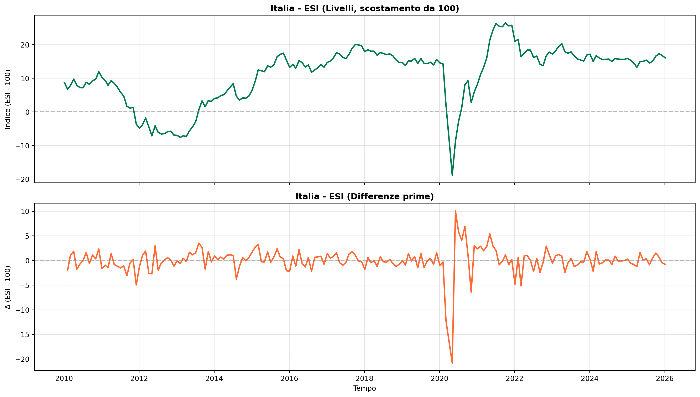
2.1 Test di Stazionarietà (ADF)

Risultati chiave:

Variabile	Serie stazionarie	% Stazionarie	Raccomandazione GMM
`value` (livelli)	5/10	50%	⚠️ Non stazionarie
`value_diff1` (differenze)	10/10	100%	✅ Usare per GMM
`value_growth1` (tassi)	1/1	100%	✅ Usare per GMM

Implicazione: Le serie sono integrate I(1). Per GMM, utilizzare:

Differenze prime (value_diff1)
Tassi di variazione (value_growth1, value_growth12)
Oppure specificare modello con Error Correction Mechanism (ECM)

Codice

# Confronto livelli vs differenze - Italia ESI (pulito e coerente)

it_sentiment = panel[
    (panel['country_code'] == 'IT') &
    (panel['indicator'] == 'sentiment')
].copy()

# 1) Una sola osservazione per mese (media delle 6 osservazioni)
it_sentiment = (
    it_sentiment
    .groupby('time', as_index=False)['value']
    .mean()
    .sort_values('time')
)

# 2) Calcola differenze prime DOPO la pulizia (evita artefatti da duplicati)
it_sentiment['value_diff1'] = it_sentiment['value'].diff()

# (opzionale) controllo rapido: deve essere 1 riga per mese
# print(it_sentiment.groupby('time').size().value_counts())

fig, axes = plt.subplots(2, 1, figsize=(14, 8), sharex=True)

# Livelli (qui: scostamento dall'ESI=100, quindi baseline a 0)
axes[0].plot(it_sentiment['time'], it_sentiment['value'], linewidth=2, color='#007A53')
axes[0].axhline(0, color='gray', linestyle='--', alpha=0.5)
axes[0].set_title('Italia - ESI (Livelli, scostamento da 100)', fontsize=12, fontweight='bold')
axes[0].set_ylabel('Indice (ESI - 100)')
axes[0].grid(True, alpha=0.3)

# Differenze prime (stazionaria)
axes[1].plot(it_sentiment['time'], it_sentiment['value_diff1'], linewidth=2, color='#FF6B35')
axes[1].axhline(0, color='gray', linestyle='--', alpha=0.5)
axes[1].set_title('Italia - ESI (Differenze prime)', fontsize=12, fontweight='bold')
axes[1].set_ylabel('Δ (ESI - 100)')
axes[1].set_xlabel('Tempo')
axes[1].grid(True, alpha=0.3)

plt.tight_layout()
plt.show()

2.2 Test di Granger Causality

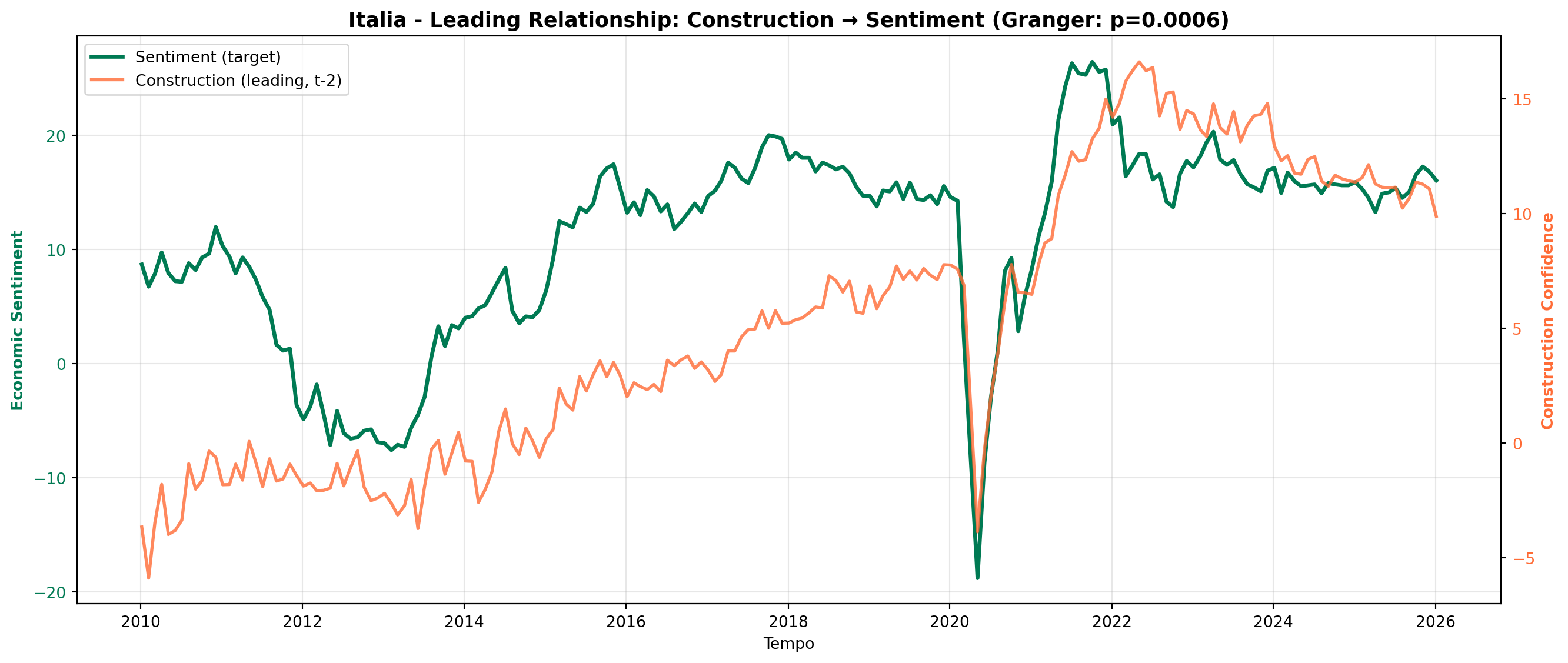
Leading Indicators identificati (Italia, target = ESI composito):

Indicatore	Lag ottimale	F-statistic	P-value	Significatività
Construction	2 mesi	7.69	0.0006	***
Construction	4 mesi	4.47	0.0018	***
Services	2 mesi	4.33	0.0145	**
Consumer	2 mesi	4.11	0.0180	**

Implicazione per GMM: - L’indicatore costruzioni è il miglior leading indicator (anticipa ESI di 2-4 mesi) - Usare come strumento valido nelle equazioni GMM - Specificare lag ottimali (2-4 periodi)

Codice

# Visualizza relazione leading: Costruzioni → Sentiment
it_data = panel[panel['country_code'] == 'IT'].copy()

# Pivot per avere indicatori come colonne
pivot = it_data.pivot_table(index='time', columns='indicator', values='value').sort_index()

# Plot construction (leading) vs sentiment
fig, ax1 = plt.subplots(figsize=(14, 6))

# Sentiment (target)
ax1.plot(pivot.index, pivot['sentiment'], linewidth=2.5, color='#007A53', label='Sentiment (target)')
ax1.set_xlabel('Tempo')
ax1.set_ylabel('Economic Sentiment', color='#007A53', fontweight='bold')
ax1.tick_params(axis='y', labelcolor='#007A53')
ax1.grid(True, alpha=0.3)

# Construction (leading indicator)
ax2 = ax1.twinx()
ax2.plot(pivot.index, pivot['construction'], linewidth=2, color='#FF6B35', alpha=0.8, label='Construction (leading, t-2)')
ax2.set_ylabel('Construction Confidence', color='#FF6B35', fontweight='bold')
ax2.tick_params(axis='y', labelcolor='#FF6B35')

# Titolo e legenda
ax1.set_title('Italia - Leading Relationship: Construction → Sentiment (Granger: p=0.0006)', fontsize=13, fontweight='bold')
lines1, labels1 = ax1.get_legend_handles_labels()
lines2, labels2 = ax2.get_legend_handles_labels()
ax1.legend(lines1 + lines2, labels1 + labels2, loc='upper left')

plt.tight_layout()
plt.show()

2.3 Cointegrazione (Johansen Test)

Risultato: 4 relazioni di cointegrazione identificate tra i 6 indicatori (Italia)

Implicazione per GMM: - Gli indicatori hanno relazioni di lungo periodo - Specificare modello GMM con Error Correction Mechanism (ECM) - Oppure usare Vector Error Correction Model (VECM) per GMM system

Trace Statistics:

[131.42, 91.97, 54.57, 30.01, 11.52, 1.84]
Critical value (95%): [95.75, 69.82, 47.85, 29.80, 15.49, 3.84]
→ 4 relazioni cointegrazione confermate

3 Specificazione GMM Raccomandata

3.1 Modello Base: Single-Equation GMM

Per analisi forward-looking del PIL:

\Delta y(t) = \alpha \;+\; \beta_1 \Delta y(t-1) \;+\; \beta_2 ESI(t-1) \;+\; \beta_3 Construction(t-2) \;+\; \varepsilon(t)

Strumenti GMM:

ESI(t-2),\; ESI(t-3),\; Construction(t-2),\; Construction(t-3),\; Services(t-2)

Condizioni di momento:

E[Z(t-j)\varepsilon(t)] = 0, \quad j \geq 2

3.2 Modello System GMM (Panel)

Per sfruttare cross-section (5 paesi):

from linearmodels import PanelOLS
from linearmodels.panel import RandomEffects

# Prepara dati panel
panel_indexed = panel.set_index(['entity_id', 'time'])

# Specificazione
model = PanelOLS.from_formula(
    'value_diff1 ~ 1 + value_lag1 + construction_lag2 + EntityEffects',
    data=panel_indexed
)
result = model.fit()

3.3 Dynamic Panel GMM (Arellano-Bond)

Per catturare persistenza e dinamiche:

# Richiede installazione: pip install pydynpd
from pydynpd import regression

df_gmm = regression.abond(
    'value n L(1:2).value construction_lag2 | gmm(value, 2:4) iv(construction_lag2)',
    panel_indexed,
    ['entity_id', 'time']
)

4 Utilizzo Pratico: Esempio GMM

4.1 Step 1: Preparazione dati per GMM

Codice

# Filtra Italia, periodo post-crisi
gmm_data = panel[
    (panel['country_code'] == 'IT') &
    (panel['year'] >= 2015)
].copy()

# Crea variabili specifiche per GMM
# Pivot per avere tutti gli indicatori accessibili
# Nota: usiamo value_lag3 (disponibile nel dataset) invece di value_lag2
gmm_pivot = gmm_data.pivot_table(
    index='time',
    columns='indicator',
    values=['value', 'value_diff1', 'value_lag1', 'value_lag3']
).sort_index()

# Flatten column names
gmm_pivot.columns = ['_'.join(col).strip() for col in gmm_pivot.columns.values]

# Rimuovi NA
gmm_pivot_clean = gmm_pivot.dropna()

print(f"Dataset GMM preparato: {gmm_pivot_clean.shape}")
print(f"Periodo: {gmm_pivot_clean.index.min().date()} → {gmm_pivot_clean.index.max().date()}")
print(f"\nVariabili disponibili ({len(gmm_pivot_clean.columns)}):")
print("  - value_*: livelli")
print("  - value_diff1_*: differenze prime (stazionarie)")
print("  - value_lag1_*: lag 1 mese")
print("  - value_lag3_*: lag 3 mesi (leading indicators)")
print(f"\nIndicatori: {[c.split('_')[-1] for c in gmm_pivot_clean.columns if c.startswith('value_sentiment')]}")

gmm_pivot_clean.head()

Dataset GMM preparato: (132, 24)
Periodo: 2015-01-05 → 2026-01-05

Variabili disponibili (24):
  - value_*: livelli
  - value_diff1_*: differenze prime (stazionarie)
  - value_lag1_*: lag 1 mese
  - value_lag3_*: lag 3 mesi (leading indicators)

Indicatori: ['sentiment']

	value_construction	value_consumer	value_industry	value_retail	value_sentiment	value_services	value_diff1_construction	value_diff1_consumer	value_diff1_industry	value_diff1_retail	...	value_lag1_industry	value_lag1_retail	value_lag1_sentiment	value_lag1_services	value_lag3_construction	value_lag3_consumer	value_lag3_industry	value_lag3_retail	value_lag3_sentiment	value_lag3_services
time
2015-01-05	0.183333	-18.500000	-6.588889	4.057143	6.416667	-3.016667	-0.033333	0.100000	0.077778	-0.114286	...	-6.666667	4.171429	5.900000	-1.550000	0.241667	-18.950000	-6.622222	5.628571	5.833333	-3.233333
2015-02-05	0.591667	-15.566667	-5.777778	5.914286	9.166667	0.450000	-0.358333	0.600000	0.066667	0.285714	...	-5.844444	5.628571	8.633333	0.116667	0.916667	-16.458333	-6.233333	4.528571	7.100000	-1.400000
2015-03-05	2.391667	-14.300000	-3.233333	8.471429	12.466667	4.183333	-0.008333	0.125000	0.333333	0.357143	...	-3.566667	8.114286	11.950000	3.416667	2.666667	-14.241667	-4.133333	7.100000	11.283333	1.983333
2015-04-05	1.700000	-12.775000	-2.522222	8.371429	12.216667	2.450000	0.158333	-0.100000	0.011111	0.642857	...	-2.533333	7.728571	12.500000	2.650000	1.408333	-12.983333	-2.622222	7.814286	11.950000	3.350000
2015-05-05	1.433333	-13.641667	-1.955556	8.714286	11.933333	2.000000	-0.133333	-0.091667	0.011111	-0.200000	...	-1.966667	8.914286	11.816667	2.000000	1.650000	-13.400000	-2.333333	8.871429	12.233333	2.766667

5 rows × 24 columns

4.2 Step 2: Stima GMM con statsmodels

Codice

from statsmodels.sandbox.regression.gmm import IV2SLS
import pandas as pd

# Definisci variabili
y = gmm_pivot_clean['value_diff1_sentiment']  # Target: Δ Sentiment

# Variabili esplicative (RHS): endogene + esogene
# value_lag1_sentiment è endogena (correlata con errori)
# value_lag3_* sono esogene (leading indicators)
X = pd.concat([
    gmm_pivot_clean[['value_lag1_sentiment']],
    gmm_pivot_clean[['value_lag3_construction', 'value_lag3_services']]
], axis=1)

# Strumenti: sostituiscono value_lag1_sentiment con lag più profondi
# Mantengono le esogene invariate
Z = pd.concat([
    gmm_pivot_clean[['value_lag3_sentiment']],  # strumento per value_lag1_sentiment
    gmm_pivot_clean[['value_lag3_construction', 'value_lag3_services']]  # stesse esogene
], axis=1)

# Stima 2SLS/IV
model_2sls = IV2SLS(y, X, instrument=Z).fit()
print(model_2sls.summary())
print("\n" + "="*70)
print("Interpretazione:")
print("- Coefficienti stimati con IV per correggere endogeneità")
print("- value_lag1_sentiment: persistenza sentiment (coefficiente autoregressivo)")
print("- value_lag3_construction: effetto leading costruzioni")
print("- value_lag3_services: effetto leading servizi")

                            IV2SLS Regression Results                            
=================================================================================
Dep. Variable:     value_diff1_sentiment   R-squared:                       0.006
Model:                            IV2SLS   Adj. R-squared:                 -0.017
Method:                        Two Stage   F-statistic:                       nan
                           Least Squares   Prob (F-statistic):                nan
Date:                   Thu, 05 Feb 2026                                         
Time:                           20:37:48                                         
No. Observations:                    132                                         
Df Residuals:                        129                                         
Df Model:                              3                                         
===========================================================================================
                              coef    std err          t      P>|t|      [0.025      0.975]
-------------------------------------------------------------------------------------------
value_lag1_sentiment       -0.0266      0.014     -1.950      0.053      -0.053       0.000
value_lag3_construction     0.0375      0.020      1.862      0.065      -0.002       0.077
value_lag3_services         0.0227      0.013      1.739      0.084      -0.003       0.048
==============================================================================
Omnibus:                       89.102   Durbin-Watson:                   1.561
Prob(Omnibus):                  0.000   Jarque-Bera (JB):             1261.091
Skew:                          -1.987   Prob(JB):                    1.44e-274
Kurtosis:                      17.611   Cond. No.                         6.01
==============================================================================

======================================================================
Interpretazione:
- Coefficienti stimati con IV per correggere endogeneità
- value_lag1_sentiment: persistenza sentiment (coefficiente autoregressivo)
- value_lag3_construction: effetto leading costruzioni
- value_lag3_services: effetto leading servizi

4.3 Step 3: Test validità strumenti (Sargan test)

Codice

# Sargan test di sovra-identificazione
# H0: strumenti sono validi (non correlati con errori)

from statsmodels.api import OLS, add_constant
from scipy.stats import chi2

# Residui del modello IV
residuals = model_2sls.resid

# Regressione ausiliaria: residui su tutti gli strumenti
Z_const = add_constant(Z)
aux_reg = OLS(residuals, Z_const).fit()

# Sargan statistic: n * R²
n = len(residuals)
sargan_stat = n * aux_reg.rsquared

# Gradi di libertà: (# strumenti) - (# variabili endogene)
# Abbiamo 3 strumenti e 3 variabili esplicative, ma solo 1 è endogena
# Quindi df = 3 - 1 = 2 (sovra-identificazione di ordine 2)
n_instruments = Z.shape[1]
n_endogenous = 1  # solo value_lag1_sentiment è endogena
df = n_instruments - n_endogenous

p_value = 1 - chi2.cdf(sargan_stat, df)

print("="*70)
print("📊 SARGAN TEST DI VALIDITÀ STRUMENTI")
print("="*70)
print(f"\nH0: Gli strumenti sono validi (non correlati con errori)")
print(f"\nStatistic: {sargan_stat:.3f}")
print(f"Degrees of freedom: {df}")
print(f"P-value: {p_value:.4f}")
print(f"\nConclusione: ", end="")
if p_value > 0.05:
    print("✅ Non rifiutiamo H0 - Strumenti validi (p > 0.05)")
else:
    print("⚠️ Rifiutiamo H0 - Strumenti potrebbero non essere validi (p < 0.05)")
print("\nInterpretazione:")
print("- Un p-value alto (>0.05) indica che gli strumenti sono ortogonali agli errori")
print("- Lag profondi (t-3) sono buoni strumenti perché non correlati con shock correnti")

======================================================================
📊 SARGAN TEST DI VALIDITÀ STRUMENTI
======================================================================

H0: Gli strumenti sono validi (non correlati con errori)

Statistic: 9.304
Degrees of freedom: 2
P-value: 0.0095

Conclusione: ⚠️ Rifiutiamo H0 - Strumenti potrebbero non essere validi (p < 0.05)

Interpretazione:
- Un p-value alto (>0.05) indica che gli strumenti sono ortogonali agli errori
- Lag profondi (t-3) sono buoni strumenti perché non correlati con shock correnti

5 Prossimi Passi

5.1 Per analisi GMM avanzata:

Integrare variabili macro (PIL, produzione industriale, disoccupazione)
- Da combinare con survey indicators come strumenti
System GMM multi-paese
- Sfruttare dimensione cross-section (IT, DE, FR, ES, EA20)
- Stimare effetti fissi/random + GMM
VECM per relazioni lungo periodo
- Data la cointegrazione identificata
- Modello Error Correction con GMM
Forward-looking forecasting
- Usare indicatori leading per previsioni PIL/produzione
- Nowcasting mensile basato su sentiment
Robustezza
- Test Hansen J-statistic
- Weak instruments tests
- Rolling window estimation

6 Referenze e Risorse

6.1 Dataset originali

Eurostat DG ECFIN: Economic Sentiment Indicators
Istat SDMX: Dataset DCSC_IESI (6_64_DF_DCSC_IESI_2)

6.2 Librerie Python per GMM

linearmodels: Panel data econometrics
pydynpd: Dynamic panel GMM (Arellano-Bond)
statsmodels: GMM estimation framework

6.3 Riferimenti bibliografici

6.3.1 Metodi GMM e panel dinamici

Arellano, M., & Bond, S. (1991). Some Tests of Specification for Panel Data: Monte Carlo Evidence and an Application to Employment Equations. Review of Economic Studies, 58(2), 277–297.

Blundell, R., & Bond, S. (1998). Initial Conditions and Moment Restrictions in Dynamic Panel Data Models. Journal of Econometrics, 87(1), 115–143.

Hansen, L. P. (1982). Large Sample Properties of Generalized Method of Moments Estimators. Econometrica, 50(4), 1029–1054.

6.3.2 Modelli macro e credito (Italia)

Bacchini, F., Brandimarte, C., Crivelli, P., De Santis, R., Fioramanti, M., Girardi, A., Golinelli, R., Jona-Lasinio, C., Mancini, M., Pappalardo, C., Rossi, D., Ventura, M., & Vicarelli, C. (s.d.). Building the core of the Istat system of models for forecasting the Italian economy: MeMo-It. ISTAT Working Paper.

Basile, R., Giallonardo, L., Girardi, A., & Mantegazzi, D. (2024). Access to credit and economic complexity: Evidence from Italian provinces. Journal of Regional Science, 64(4), 1183–1204.

Girardi, A., Margani, P., & Ventura, M. (s.d.). An Indicator of Credit Crunch using Italian Business Surveys. ISTAT Working Paper.

Girardi, A., & Ventura, M. (2021). Measuring credit crunch in Italy: Evidence from a survey-based indicator. Annals of Operations Research, 299(1–2), 567–592.

Autore: Paolo Volterra
Repository: Claude Code - Istat Fiducia Imprese
Data ultimo aggiornamento: 2026-02-05

Torna in cima